Slender plane beam element for large displacements and rotations

Consider an arbitrary element of a planar beam structure, which, in the unloaded state is in the reference position C0 (Fig. 5.1) defined by the coordinates of the nodal points i and j.

After loading, the beam was moved to position C1, and the displacement components of the nodal points that arose during this movement were arranged into a vector

${{\mathbf{u}}_{e}}={{\left[ \begin{matrix} {{u}_{i}} & {{v}_{i}} & {{\varphi }_{i}} & {{u}_{j}} & {{v}_{j}} & {{\varphi }_{j}} \\ \end{matrix} \right]}^{T}}$

(5.1)

The removed parts of the structure act with force resultants at the end points of the beam, organized into a vector of the element’s internal nodal forces

\[{{\mathbf{q}}_{e}}={{\left[ \begin{matrix} {{Q}_{ix}} & {{Q}_{iy}} & {{M}_{i}} & {{Q}_{jx}} & {{Q}_{jy}} & {{M}_{j}} \\ \end{matrix} \right]}^{T}}\]

(5.2)

The procedure for determining the basic matrices of the element is analogous to that used when solving the same problem for a plane truss element (Ch.4). We need to express the terms ${{\mathbf{q}}_{e}}$ as functions of the components ${{\mathbf{u}}_{e}}$ from relation (4.6)

\[{{\mathbf{q}}_{e}}=\frac{\partial {{U}_{e}}}{\partial {{\mathbf{u}}_{e}}}\]

(5.3)

This allows to assemble the equilibrium equations of the nodes and the tangential element matrix from the relation

\[\mathbf{K}_{T}^{e}=\frac{\partial {{\mathbf{q}}_{e}}}{\partial {{\mathbf{u}}_{e}}}\]

(5.4)

The tangential element matrices can then be combined into the resulting tangential matrix of the structure and used in an iterative process to solve of the whole structure deformation.

When determining the strain energy of the beam, it is advantageous to use the local coordinate system of the element $\bar{x}$,$\bar{y}$ , which is tied to the movement of the element, in which the nodal force components represent the axial force N = Nj = -Ni and transverse forces Ti , Tj . The nodal bending moments ${{M}_{i}}$, ${{M}_{j}}$ were identical in both the coordinate systems.

We will proceed from the assumption that we are dealing with a slender beam in which the energy of the shear stresses can be neglected. Thus, the transverse forces do not contribute to the deformation of the beam, and the local vector of the element deformation forces has only three components:

\[{{\mathbf{\bar{q}}}_{e}}={{\left[ \begin{matrix} N & {{M}_{i}} & {{M}_{j}} \\ \end{matrix} \right]}^{T}}\]

(5.5)

Because we do not consider external loads on the element (external loads will be applied only to the nodes, which we have virtually separated from the element), the transverse forces are equal in magnitude T = Ti = -Tj ; of course, the nodal moments of the element are linked by the moment equilibrium condition with the transverse force

\[{{T}_{i}}=\left( {{M}_{i}}+{{M}_{j}} \right)/L\]

(5.6)

In the local coordinate system, the relationships between the nodal forces and displacements (Fig. 5.1), which contribute to the deformation of the beam, follow the equations known from the linear stiffness matrix of the element

${{\mathbf{\bar{q}}}_{e}}=\left[ \begin{matrix} N \\ {{M}_{i}} \\ {{M}_{j}} \\ \end{matrix} \right]=\left[ \begin{matrix} \frac{{{E}_{0}}{{S}_{0}}}{{{L}_{0}}} & 0 & 0 \\ 0 & \frac{4{{E}_{0}}{{I}_{0}}}{{{L}_{0}}} & \frac{2{{E}_{0}}{{I}_{0}}}{{{L}_{0}}} \\ 0 & \frac{2{{E}_{0}}{{I}_{0}}}{{{L}_{0}}} & \frac{4{{E}_{0}}{{I}_{0}}}{{{L}_{0}}} \\ L-{{L}_{0}} \\ {{{\bar{\varphi }}}_{i}} \\ {{{\bar{\varphi }}}_{j}} \\ \end{matrix} \right]=\mathbf{D}{{\mathbf{\bar{u}}}_{e}}$

(5.7)

where ${{E}_{0}}$ is the modulus of elasticity of the material, S0 is the cross-sectional area, and ${{I}_{0}}$ quadratic moment of the beam cross-section.

The internal nodal forces perform work during beam deformation, and the magnitude of this work is identical to the strain energy accumulated in the deformed element

\[{{U}_{e}}={{U}_{N}}+{{U}_{M}}=\frac{1}{2}N\left( L-{{L}_{0}} \right)+\frac{1}{2}\left( {{M}_{i}}{{{\bar{\varphi }}}_{i}}+{{M}_{j}}{{{\bar{\varphi }}}_{j}} \right)\]

(5.8)

Using , the nodal forces of the element in can be eliminated, thus allowing the use of the deformation formulation of the element via the following relationships:

\[{{U}_{N}}=\frac{1}{2}N\left( L-{{L}_{0}} \right)=\frac{1}{2}\sigma {{S}_{0}}\left( L-{{L}_{0}} \right)=\frac{1}{2}{{E}_{0}}{{\varepsilon }_{ing}}{{S}_{0}}\left( L-{{L}_{0}} \right)=\frac{1}{2}{{E}_{0}}{{S}_{0}}{{L}_{0}}\varepsilon _{ing}^{2}\]

(5.9)

\[{{U}_{M}}={{U}_{{{M}_{i}}}}+{{U}_{{{M}_{j}}}}=\frac{1}{2}{{M}_{i}}{{\bar{\varphi }}_{i}}+\frac{1}{2}{{M}_{j}}{{\bar{\varphi }}_{j}}=\frac{1}{2}\left( \frac{4{{E}_{0}}{{I}_{0}}}{{{L}_{0}}}{{{\bar{\varphi }}}_{i}}+\frac{2{{E}_{0}}{{I}_{0}}}{{{L}_{0}}}{{{\bar{\varphi }}}_{j}} \right){{\bar{\varphi }}_{i}}+\frac{1}{2}\left( \frac{2{{E}_{0}}{{I}_{0}}}{{{L}_{0}}}{{{\bar{\varphi }}}_{i}}+\frac{4{{E}_{0}}{{I}_{0}}}{{{L}_{0}}}{{{\bar{\varphi }}}_{j}} \right){{\bar{\varphi }}_{j}}\]

(5.10)

Quantities ${{\varepsilon }_{ing}}$, ${{\bar{\varphi }}_{i}}$ and ${{\bar{\varphi }}_{j}}$ include the global nodal displacements of the element, and if we want to apply and it is necessary to express these relationships. For simplicity, it is advantageous to search for the vector of nodal forces in the form

\[{{\mathbf{q}}_{e}}={{\mathbf{q}}_{N}}+{{\mathbf{q}}_{{{M}_{i}}}}+{{\mathbf{q}}_{{{M}_{j}}}}=\frac{\partial {{U}_{N}}}{\partial {{\mathbf{u}}_{e}}}+\frac{\partial {{U}_{{{M}_{i}}}}}{\partial {{\mathbf{u}}_{e}}}+\frac{\partial {{U}_{{{M}_{j}}}}}{\partial {{\mathbf{u}}_{e}}}\]

(5.11)

so that we can derive the element energies separately. The calculation ${{\mathbf{q}}_{N}}$ is analogous to the calculation of this vector for the truss element (Ch.4) differences arise only from the fact that here, we use the engineering strain of the beam instead of Green’s strain

\[{{\mathbf{q}}_{N}}=\frac{\partial {{U}_{N}}}{\partial {{\mathbf{u}}_{e}}}={{E}_{0}}{{S}_{0}}{{L}_{0}}{{\varepsilon }_{ing}}\frac{\partial {{\varepsilon }_{ing}}}{\partial {{\mathbf{u}}_{e}}}=\sigma {{S}_{0}}{{L}_{0}}\frac{\partial {{\varepsilon }_{ing}}}{\partial {{\mathbf{u}}_{e}}}=N{{L}_{0}}\frac{\partial \left( \frac{L-{{L}_{0}}}{{{L}_{0}}} \right)}{\partial {{\mathbf{u}}_{e}}}=N\frac{\partial L}{\partial {{\mathbf{u}}_{e}}}\]

(5.12)

$L=\sqrt{{{\left( {{X}_{ji}}+{{u}_{ji}} \right)}^{2}}+{{\left( {{Y}_{ji}}+{{v}_{ji}} \right)}^{2}}}$

\[{{\mathbf{q}}_{N}}=N{{\left[ \begin{matrix} -\cos \beta & -\sin \beta & 0 & \cos \beta & \sin \beta & 0 \\ \end{matrix} \right]}^{T}}\]

(5.13)

$\cos \beta =\frac{{{X}_{ji}}+{{u}_{ji}}}{L}$, $\sin \beta =\frac{{{Y}_{ji}}+{{v}_{ji}}}{L}$

The variables with double indices express the differences in the respective quantities at nodes j and i.

The derivation of the remaining two columns of the nodal force vector is not presented here because of its length (see e.g. [1]); its final form is

\[\mathbf{q}_e = \mathbf{B}^T \bar{\mathbf{q}}_e = \begin{bmatrix} -\cos\beta & -\frac{\sin\beta}{L} & -\frac{\sin\beta}{L} \\ -\sin\beta & \frac{\cos\beta}{L} & \frac{\cos\beta}{L} \\ 0 & 1 & 0 \\ \cos\beta & \frac{\sin\beta}{L} & \frac{\sin\beta}{L} \\ \sin\beta & -\frac{\cos\beta}{L} & -\frac{\cos\beta}{L} \\ 0 & 0 & 1 \end{bmatrix} \begin{bmatrix} N \\ M_i \\ M_j \end{bmatrix}\]

(5.14)

In this relation, it is still necessary to determine the dependence of nodal forces N, ${{M}_{i}}$ and ${{M}_{j}}$ on the global displacements of the element, that is, to express $L-{{L}_{0}}$, ${{\bar{\varphi }}_{i}}$ and ${{\bar{\varphi }}_{j}}$ in the equations . Expressing the axial change in the length of the beam is straightforward because

${{L}_{0}}=\sqrt{X_{ji}^{2}+Y_{ji}^{2}};\quad \quad L=\sqrt{{{\left( X_{ji}^{{}}+{{u}_{ji}} \right)}^{2}}+{{\left( Y_{ji}^{{}}+{{v}_{ji}} \right)}^{2}}}$

\[{{\bar{\varphi }}_{i}}={{\varphi }_{i}}-\alpha ;\quad \quad {{\bar{\varphi }}_{j}}={{\varphi }_{j}}-\alpha \]

(5.15)

\[\sin \left( \alpha +\delta \right)=\sin \beta ;\quad \quad \cos \left( \alpha +\delta \right)=\cos \beta \]

(5.16)

where $\sin \delta ={{Y}_{ji}}/{{L}_{0}},\ \ \cos \delta ={{X}_{ji}}/{{L}_{0}}$. By expanding the known trigonometric relationships for the sum of two angles, we obtain two equations, from which we obtain:

\[\sin \alpha =\frac{1}{L{{L}_{0}}}\left( {{X}_{ji}}{{v}_{ji}}-{{Y}_{ji}}{{u}_{ji}} \right)\text{;}\quad \quad \cos \alpha =\frac{1}{L{{L}_{0}}}\left[ {{X}_{ji}}\left( {{X}_{ji}}+{{u}_{ji}} \right)+{{Y}_{ji}}\left( {{Y}_{ji}}+{{v}_{ji}} \right) \right]\]

(5.17)

\[\alpha =\arctan \left( \frac{{{X}_{ji}}{{v}_{ji}}-{{Y}_{ji}}{{u}_{ji}}}{{{X}_{ji}}\left( {{X}_{ji}}+{{u}_{ji}} \right)+{{Y}_{ji}}\left( {{Y}_{ji}}+{{v}_{ji}} \right)} \right)\]

(5.18)

From the known vector of the element’s nodal forces, it is now possible to determine the element’s tangential matrix according to (9.4). We present the results in the simplest form

\[\mathbf{K}_{T}^{e}=\mathbf{K}_{M}^{e}+\mathbf{K}_{G}^{e}={{\mathbf{B}}^{T}}\mathbf{DB}+\mathbf{K}_{GN}^{e}+\mathbf{K}_{GM}^{e}\] where $\mathbf{K}_{GN}^{e}=\frac{N}{30L}\left[ \begin{matrix} 36{{\sin }^{2}}\beta & -18\sin 2\,\beta & -3L\sin \beta & -36{{\sin }^{2}}\beta & 18\sin 2\,\beta & -3L\sin \beta \\ {} & 36{{\cos }^{2}}\beta & 3L\cos \beta & 18\sin 2\,\beta & -36{{\cos }^{2}}\beta & 3L\cos \beta \\ {} & {} & 4{{L}^{2}} & 3L\sin \beta & -3L\cos \beta & -{{L}^{2}} \\ {} & {} & {} & 36{{\sin }^{2}}\beta & -18\sin 2\,\beta & 3L\sin \beta \\ {} & SYM & {} & {} & 36{{\cos }^{2}}\beta & -3L\cos \beta \\ {} & {} & {} & {} & {} & 4{{L}^{2}} \\ \end{matrix} \right]$ , \[\mathbf{K}_{\text{GM}}^{\text{e}}=\frac{\text{T}}{\text{L}}\left[ \begin{matrix} \sin 2\,\beta & -\cos 2\,\beta & 0 & -\sin 2\,\beta & \cos 2\,\beta & 0 \\ {} & \sin 2\,\beta & 0 & \cos 2\,\beta & \sin 2\,\beta & 0 \\ {} & {} & 0 & 0 & 0 & 0 \\ {} & {} & {} & \sin 2\,\beta & -\cos 2\,\beta & 0 \\ {} & \text{SYM} & {} & {} & -\sin 2\,\beta & 0 \\ {} & {} & {} & {} & {} & 0 \\ \end{matrix} \right]\]

(5.19)

The material stiffness matrix in (5.19) $\mathbf{K}_M^e = \mathbf{B}^T \mathbf{D} \mathbf{B}$ expresses the material and dimensional stiffness of the element; it is essentially the stiffness matrix of the element in the local coordinate system transformed into the global system, and it represents the standard stiffness matrix for the equilibrium position of the element. The geometric stiffness matrix of the element is formed by the sum of the matrix $\mathbf{K}_{GN}^e$ (the influence of the axial force on the stiffness of the beam) and $\mathbf{K}_{GM}^e$ (the influence of nodal moments).

Example 5.1 For the planar beam structure in the figure, calculate the horizontal and vertical components of the displacement of node 3 when given: a = 1000 mm, square cross-sectional area A0 = 100 mm2, E0 = 200 000 MPa, I0 = $\text{1}{{\text{0}}^{\text{4}}}\text{/12=833}\text{.33}$ mm4 and F = 50 N.

Program Mathematica 7 is constructed for single-purpose use, only for the needs of this example; its modification to compute multiple-element examples is straightforward, but this is not its primary intention. Above all, it serves as an illustrative demonstration of the method for using matrices of the nonlinear beam element.

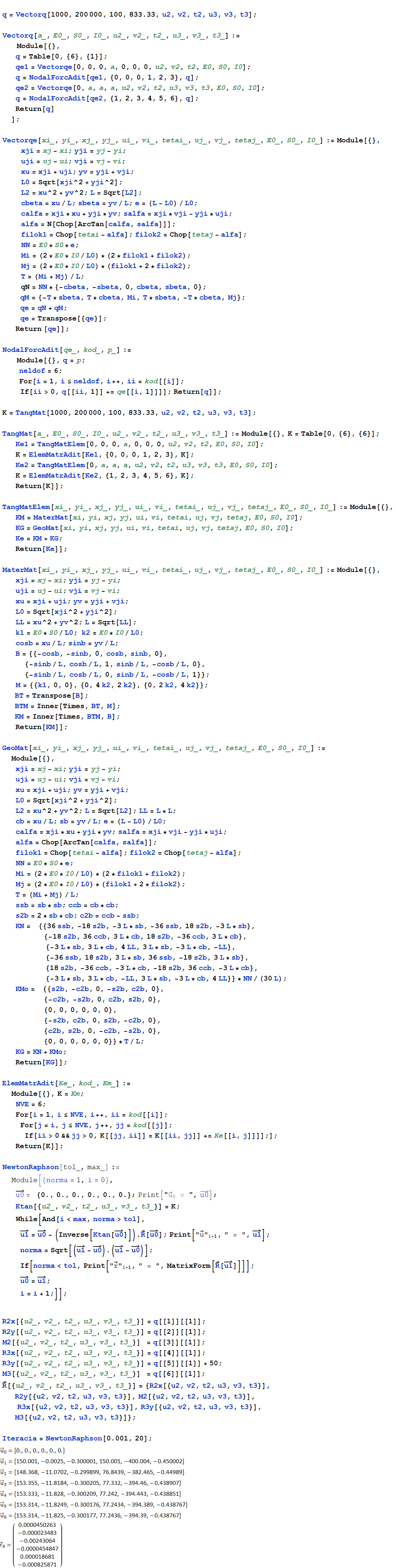
Results of the iterative process (${{u}_{2}},{{v}_{2}},{{\varphi }_{2}},{{u}_{3}},{{v}_{3}},{{\varphi }_{3}}$)and the vector of unbalanced forces after meeting the convergence criterion

$\vec{u}_0 = \{0., 0., 0., 0., 0., 0.\}$

$\vec{u}_1 = \{150.001, -0.0025, -0.300001, 150.001, -400.004, -0.450002\}$

$\vec{u}_2 = \{148.368, -11.0702, -0.299899, 76.8439, -382.465, -0.44989\}$

$\vec{u}_3 = \{153.355, -11.8184, -0.300205, 77.332, -394.46, -0.438907\}$

$\vec{u}_4 = \{153.333, -11.828, -0.300209, 77.242, -394.443, -0.438851\}$

$\vec{u}_5 = \{153.314, -11.8249, -0.300176, 77.2434, -394.389, -0.438767\}$

$\vec{u}_6 = \{153.314, -11.825, -0.300177, 77.2436, -394.39, -0.438767\}$

The displacement components of node No. 3 are: ${{u}_{3}}=$ 77.2 mm; ${{v}_{3}}=$ - 394.4 mm. The second line (1st iteration) presents the results of the linear solution of the problem. We also entered the example into the ANSYS Mechanical APDL program; its results are presented in the attached Video 5.1. Using the ANSYS program, we obtained the following displacement components for node No. 3: ${{u}_{3}}=$ xxx mm; ${{v}_{3}}=$ - xxx mm. Minor deviations from the previous calculation were caused by the fact that in ANSYS the element 188 is formulated differently. (The BEAM188 is suitable for analyzing slender to moderately stubby/thick beam structures. The element is based on Timoshenko beam theory which includes shear-deformation effects.) When displaying the solution with only two elements, we only obtained a straight-line connection of the three displaced nodes. In the real numerical analysis of beam (frame) structures using FEM, it is necessary to divide them into more than one element. After such a calculation, we obtained realistic results in the example for vertical node displacements:

Slender plane beam element for large displacements and rotations (DRAFT)